When trying to understand the low temperature asymptotic of entropic regularization in optimal transport, Gibbs measures naturally appear and their Taylor expansions are needed. This can be reduced to expanding w.r.t. $\varepsilon$ around $\varepsilon = 0$ the following type of integral $$ \mathcal L(\varepsilon) = \int_{\mathbb R^d} \phantom{1} e^{-u(x)/ε}\phantom{1} \rho(x)dx$$ where $u$ is a function that attains its minimum on a subset of $\mathbb R^d$ and $\rho(x)$ is a positive function. Such integrals are ubiquitous in many different fields, inside and outside mathematics. The Laplace method answers this question. For the reader interested in machine learning and statistical applications of the Laplace method, we refer to the nice post of Francis Bach (at the bottom, don’t miss the very playful discussion between Napoléon and Laplace).
For instance, when this subset is a single point, say w.l.o.g. $0$, at which the function $u$ has a nonsingular hessian. Thus, when possible, the Taylor expansion of $u$ at $0$ is $$u(x) = u(0) + \frac 12 \langle Hx,x \rangle + o(| x - x_*|^2)\,,$$ with $H$ the Hessian matrix of $u$ at $0$. This suggests that the integral above can be approximated by a Gaussian integral to get $$ \mathcal L(\varepsilon) \approx \frac{(2\pi\varepsilon )^{\frac d 2}}{\sqrt{det(H)}}e^{-\frac{u(0)}{\varepsilon}} \rho(0)\,. $$ Different proofs are available. One of them consists in using Morse lemma to make a change of variable so that $u \circ \varphi(x) = u(0) + \frac 12 \langle Hx,x \rangle$ in a neighborhood of $0$. The change of variable affects the density $\rho$, which can then be Taylor expanded so that one is left with moments of Gaussian (the rest of the integral outside this neighborhood can be neglected). Another strategy of proof consists in Taylor expanding the exponential with the remainder to the quadratic approximation and Taylor expanding the density as well. The formula then reduces to Gaussian integrals and Isserli’s formula is useful there.
In the same setting as above but with $\rho(x) = 1$, let us look at the first-order Laplace expansion to see how complicated it gets. Hereafter, terms involving $u$ on the right-hand side are evaluated at $0$, see the book of [McCullagh], $$ \int_{\mathbb R^d} \frac{e^{-u(x)/\varepsilon}}{(2\pi\varepsilon)^{d/2}} \,dx = \frac{e^{-u/\varepsilon}}{\sqrt{det (u_{ij})}}\bigg(1 + \frac{\varepsilon}{8} u_{ijk}u_{\ell mn}u^{ij}u^{k\ell}u^{mn} +\frac{\varepsilon}{12} u_{ijk}u_{\ell mn} u^{i\ell} u^{jm} u^{kn} - \frac{\varepsilon}{8} u_{ijk\ell}u^{ij}u^{k\ell}+ O(\varepsilon^2)\bigg)\,. $$ This formula is already quite complicated and does not even involve a general density $\rho$. In some settings, this formula is not particularly easy to manipulate. It would be much nicer to have objects such as divergence, gradients and tensors in this formula in order to perform further derivations. A possible strategy is to look for a geometric formulation of this formula. Indeed, on the right-hand side, only derivatives of $u$ up to order $4$ are involved. I can now ask the (open) question of this post (please email me with any reference or answer):
Does there exist a geometric formulation of this first-order term (and higher)?
This question can be motivated by the remark that the right-hand side uses derivatives of $u$ up to order $4$ and not more and in addition, the square root factor on the Hessian of $u$ looks like a volume form for the Hessian of $u$. Indeed, if the function $u$ is smooth, it is strongly convex in a neighborhood of $0$ and defines a Hessian type of Riemannian metric. So, maybe after all, the right-hand side of this expansion might be connected with curvature terms and volume form of a particular metric.
Is this question really relevant?
It is not completely clear that a geometric formulation is necessary here. Indeed, one only needs a volume form and a function on a manifold to define the Laplace integral. By the first argument in the sketch of proof above, one deforms the function $u$ to a quadratic function, so it doesn’t seem that there is any geometric content. However, the effect of the function $u$ has been pushed into the volume form and in one dimension, appears the following kind of formulas [Bender, Chapter 5]
$$
\int_{\mathbb R} \frac{e^{-u(x)/\varepsilon}}{\sqrt{(2\pi \varepsilon)}}r(x)dx =\, \frac{e^{-u/\varepsilon}}{\sqrt{(u^{(2)})}} \bigg(r
+ \varepsilon \Big( \frac{r^{(2)}}{2u^{(2)}} - \frac{r’
u^{(3)}}{2 (u^{(2)})^2}
- \frac{r \,u^{(4)}}{8 (u^{(2)})^2} + \frac{5 r\, (u^{(3)})^2}{24 (u^{(2)})^3} \Big) + O(\varepsilon^2) \bigg)\,.
$$
As a consequence, there is still a hope one could gain insight on these terms using a more geometric approach.
In a recent work together with Flavien Léger [Léger, 2022], we propose a geometric formulation for this problem, although such a formulation might be not unique in this particular case. In fact, our main contribution does not directly apply to this case but it applies for instance when the set of minimizers of the function $u$ is a submanifold of dimension $d$ in $\mathbb R^d \times \mathbb R^d$. Such a setting appears for instance in the parametrix of the heat kernel $e^{-\frac 12 d(x,y)^2}$ on a Riemannian manifold $M\times M$. Here, one has $u = \frac 12 d(x,y)^2$ and the set of minimizer is the diagonal $\Sigma = \{ (x,x) \in M\times M \}$. This situation with two variables is also relevant in Bayesian modeling, e.g. with Gaussian priors.
In fact, our initial motivation was the understanding of entropic regularization of optimal transport and such a submanifold is embodied by the optimal transport plan when supported on the graph of a function. This situation is somehow the generic one when the cost in the optimal transportion problem is twisted, which is the case for the quadratic cost on Euclidean space. Smoothness of this submanifold involves the so-called Ma-Trudinger-Wang tensor, which is essentially the curvature tensor of a Riemannian pseudo-metric, the so-called Kim–McCann metric, which plays an important role hereafter. For the reader knowledgeable in entropic regularization of optimal transport, the optimizer of the entropic problem concentrates around the optimal transport plan and the type of integrals we have to study are of the type $$ \mathcal L(\varepsilon) = \int_{\mathbb R^d} \phantom{1} e^{-u(x,y)/ε}\phantom{1} \rho(x,y)dxdy\,, $$ where the function $u(x,y)$ defines a submanifold $\Sigma$ of minimizers that can be parametrized by either $x$ or $y$ by a diffeomorphism $(x,y(x))$ for instance. Although this setting might seem a bit intricate at first sight, it turns out that it encompasses also the classical setting of the Laplace transform mentioned above by using a translation invariant cost such as $u(x,y) = U(x-y)$ where $U$ is a function which has a unique minimum.
To briefly describe the strategy of proof, we start from the first-order multidimensional Laplace formula for which we give a proof with a quantified remainder, $$ \int_X \frac{e^{-u(x)/\varepsilon}}{(2\pi\varepsilon)^{d/2}} \,r(x)dx = \, \frac{1}{\sqrt{det(u_{ij})}}\bigg(r + \varepsilon\Big(\frac 12 u^{ij}\partial_{ij}r-\frac 12 u_{jk\ell}u^{ij}u^{k\ell}\partial_ir + \frac 18 r\,u_{ijk}u_{\ell mn}u^{ij}u^{k\ell}u^{mn}+\frac{1}{12} r\, u_{ijk}u_{\ell mn} u^{i\ell} u^{jm} u^{kn} - \frac 18 r\, u_{ijk\ell}u^{ij}u^{k\ell}\Big)\bigg)+ \varepsilon^2\,\mathcal{R}(\varepsilon)\,. $$ We further assume strong convexity in one of the variable at every point $(x,y(x))$ and we use this formula along the manifold $\Sigma$. We are left with a formula that has no particular geometric meaning. With a background in optimal transportation and a bit of practice with the Kim-McCann metric, it is slightly tempting to use it to interpret this formula in this language. This strategy works and this is the main content of the paper [Léger, 2022] to derive all the long computations necessary to show this interpretation can be achieved. Interestingly, all these computations were checked to some extent using Cadabra, which is a symbolic computation library. Let me cite their webpage:
Cadabra is a symbolic computer algebra system (CAS) designed specifically for the solution of problems encountered in field theory. It has extensive functionality for tensor computer algebra, tensor polynomial simplification including multi-term symmetries, fermions and anti-commuting variables, Clifford algebras and Fierz transformations, component computations, implicit coordinate dependence, multiple index types and many more.

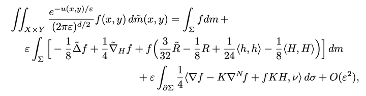
Let me try to explain this formula. In the formula above, there are two Riemannian metrics involved, $\tilde g$ and $g$. On $X\times Y$, $\tilde g$ is the (pseudo-Riemannian) metric introduced by Kim and McCann [KimMcCann2007] which is (essentially) given by the cross-derivatives of the function $u$. Once restricted to $\Sigma$, it gives, under additional conditions, a Riemannian metric $g$. The volume forms $\tilde m, m$ are, up to rescaling, the ones induced by $\tilde g$ and $g$; $\tilde R$ and $R$ are the respective scalar curvatures of $\tilde g$ and $g$, and $\tilde \Delta$ denotes the pseudo-Riemannian Laplacian associated to $\tilde g$. Associated to $\Sigma$ considered as a submanifold of $X\times Y$, the second fundamental form is denoted by $h$ and $H$ is the mean curvature. Then, $\nabla_{!H}$ is the covariant derivative in direction $H$. The quantities $\langle h,h \rangle$ and $\langle H,H \rangle$ denote the pseudo-norms of the second fundamental form and the mean curvature, respectively. Finally, $K$ is the para-complex structure coming from the Kim–McCann geometry and $\nabla^N\,f$ is the normal component of the gradient of $f$. Taking a step back, it is expected that a neighborhood of $\Sigma$ necessarily appears in some way in the derivation of this Laplace formula. Thus, the geometry encoded by $u$ outside $\Sigma$ has to be represented in the formula. Also, it is not unexpected that intrinsic and extrinsic curvature terms of $\Sigma$ show up in this formula.
Finally, let me describe in more details this pseudo-Riemannian metric introduced by Kim and McCann. Given a cost $c(x,y)$, Kim and McCann introduced the cross-difference $$ \delta:= [c(x+\xi,y)+c(x,y+\eta)]-[c(x,y)+c(x+\xi,y+\eta)]\,, $$ which gives by Taylor expansion, $$ \delta = -D^2_{xy}c(x,y)(\xi,\eta) + o(|\xi|^2+|\eta|^2)\,. $$ This cross difference has to be nonnegative along the optimal transport plan, but it is well-defined everywhere on the product space. The Kim-McCann metric is defined by $$ \tilde g(x,y) = - \frac 12 \begin{pmatrix} 0 & D^2_{xy}c(x,y) \\ D^2_{xy}c(x,y) & 0\end{pmatrix}\,. $$ It is only a pseudo-Riemannian metric on the product space since it is not definite. However, when restricted to the the optimal transport plan it gives a standard Riemannian metric, denoted by $g$ in the formula above.
As a conclusion, this post is for me the opportunity to ask the reader for references or insight on other geometric formulations of the Laplace method, about which I am very curious.
References.
[McCullagh] Peter McCullagh, Tensor methods in statistics (Monographs on statistics and applied probability, Chapman and Hall, 1987).
[Bender1999] Carl M. Bender, Asymptotic Expansion of Integrals (Springer New York, 1999).
[Leger2022] Flavien Léger and François-Xavier Vialard, A geometric Laplace formula (ArXiv, 2022).
[KimMcCann2007] Young-Heon Kim and Robert J. McCann, Continuity, curvature, and the general covariance of optimal transportation (J. Eur. Math. Soc., 2007).