In a couple of recent papers on applied optimal transport (OT), we used the fact that the so-called semi-dual formulation of OT provides more convexity than the standard formulation of OT which is a linear programming problem (possibly infinite dimensional, see [Muzellec] or [Vacher]). In this case, this enables to obtain better stability estimates via some form of strong convexity. Let me give more details on this case: Optimal transport in its dual formulation is a linear optimization problem that aims to find two functions $f,g$ called potentials maximizing $$ \langle f,\mu\rangle + \langle g,\nu\rangle$$ under the constraint $$ f(x) + g(y) \leq c(x,y)\, \forall x,y \in D\,,$$ for two given probability measures $\mu,\nu$ on a Euclidean domain $D$. The dual pairing $\langle\cdot,\cdot\rangle$ stands for the duality between continuous functions and Radon measures. The objective function being linear, this problem is not strongly convex. To gain convexity, one can optimize on $g$ for a given $f$. This optimal $g$ is called the c-transform of $f$ and is given by $f^c(y) := \inf_{x} c(x,y) - f(x)$. Now, the resulting functional, called the semi-dual $$ J(f) = \langle f,\mu\rangle + \langle f^c,\nu\rangle\,.$$ For the cost $c(x,y) = - x \cdot y$, the semi-dual satisfies the inequality, under the assumption that $\nabla f$ is $M$-Lipschitz, $$| \nabla f - \nabla f_{\star} |_{L^2(\mu)}^2 \leq 2 M ( J(f_{\star}) - J(f)) \, , \phantom{1111} (1)$$ where $f_{\star}$ is an optimal potential, also assumed differentiable (hypothesis which is satisfied for instance if the measure $\mu$ is absolutely continuous with respect to the Lebesgue measure). Inequality (1) is a stability estimate which resembles to strong convexity. See [Vacher] for more details on this inequality.
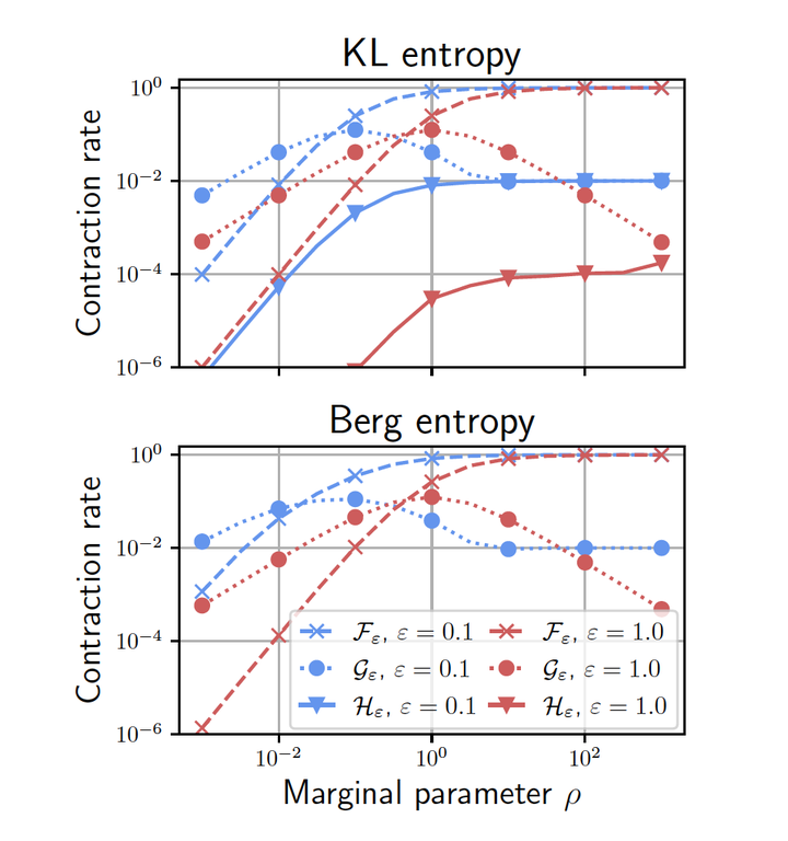
Similarly, on entropic unbalanced optimal transport, we explored the possibility of optimizing first the dual formulation with respect to a particular variable in [Séjourné]. This variable has a particular role in the optimization problem, which reads, for the case of the KL divergence, $$\sup_{f,g} -\langle 1 - e^{-f(x)},\mu(x)\rangle -\langle 1 - e^{-g(y)},\nu(y)\rangle -\varepsilon \langle e^{(f(x)+g(y)-c(x,y))/\varepsilon} - 1,\mu(x) \otimes \nu(y) \rangle \,.$$ The term involving $\varepsilon >0$ is due to the entropic regularization and one can observe that this exponential term is left unchanged under the translations $(f,g) \mapsto (f+z,g-z)$ for any constant $z \in \mathbb R$. Therefore, it is clear that there will be no effect of entropy regularization in this direction and in particular no gain in strong convexity (actually concavity in this example). Thus, it is immediate to postulate that in order to leverage the local strong convexity of $\exp$, one first needs to get rid of $c$ by optimizing on it. Interestingly, one can derive a new objective functional which turns out to have an explicit coordinate ascent algorithm (for the entropic regularization of the Gaussian-Hellinger distance) with better convergence properties than the initial Sinkhorn algorithm (coordinate ascent on the initial dual formulation). The improved convergence rate is shown on the picture above, the red (or blue) triangle curve is the improved rate of convergence for different parameter values. We refer to [Séjourné] for more details: link to article.
A simplified setting.
As seen above, optimizing on some variables can lead to strong convexity, in particular in infinite dimensions. This is well-known in optimization textbooks El Ghaoui’s course that this partial optimization step leads to Schur complement [Schur] for the Hessian of the resulting function, as detailed below. To make things simple, I consider the case of a smooth and strongly convex function $f(x,y)$ \begin{equation} f: \mathbb R^n \times \mathbb R^m \mapsto \mathbb R\,, \end{equation} on which we perform coordinate optimization on the second variable $y$. Existence of partial (i.e. with respect to $y$) minimizers is implied by strong convexity. Denote \begin{equation} y(x) := \arg \min_{y} f(x,y)\,. \end{equation} It is implicitly defined by \begin{equation} \partial_y f(x,y(x)) = 0\,. \phantom{1111} (2) \end{equation} Then, finding the minimum of $f$ is equivalent to finding the minimum of $g$ defined by \begin{equation} g(x) = f(x,y(x)) = \min_{y} f(x,y)\,, \end{equation} which is equivalent to solving the first-order condition on $g$. This equation is obtained by the envelope theorem, \begin{equation} \partial_x g(x) = \partial_x f(x,y(x))\,. \end{equation} Differentiating the previous equation and Equation (2) leads to the Hessian of $g$, $$ \nabla^2 g = \partial_{xx} g = \partial_{xx} f - \partial_{yx}f (\partial_{yy} f)^{-1} \partial_{xy}f\,, $$ which is the Schur complement of the Hessian of $f$ with respect to its block corresponding to the Hessian of $f$ w.r.t. the second variable $y$. In fact, minimizing $f$ under the constraint of Equation (2) leads to this result. More generally, this Schur complement arises in general saddlepoint problems and is used extensively in numerical optimization. Let us denote the hessian of $f$ by $$\nabla^2 f = \begin{pmatrix} \partial_{xx} f & \partial_{xy} f \\ \partial_{yx} f & \partial_{yy} f \end{pmatrix}\,,$$ and the Schur complement $\nabla^2 g$ by $\nabla^2 f / \partial_{yy} f$. The standard textbook result on Schur complement states that given the symmetric real matrix $M = \begin{pmatrix} A & B \\ B^\top & C\end{pmatrix}$ with $C$ positive definite, $M$ is positive semidefinite if and only if $M/C$ is also positive semidefinite. In our case, the direct implication reads $\nabla^2 f$ is positive semidefinite implies $\nabla^2 g$ is positive semidefinite, which we already know since partial minimization of a convex function is also convex, so the direct implication is clear in our case.
… and optimization.
Is it better to optimize on $g$ or directly on $f$ ? As such this question is not precise enough since $g$ is already an optimized version of $f$ which might be costly. Let us restrict this question to a quantitative measure of convexity and smoothness of the function $g$ in terms of that of $f$, which is directly related to the rate of convergence of first-order gradient descent.
Indeed, recall that gradient descent (or gradient flow with respect to time parameter $t$) on a smooth and strongly convex function $f$ has linear rate of convergence in $e^{-t/\kappa}$. Here, $\kappa(f)$ denotes an upper bound on the ratio $\frac{\beta}{\alpha}$ with $\alpha$ is a strong convexity parameter of $f$ and $\beta$ is a Lipschitz constant for the gradient of $f$. Therefore, it is reasonable to estimate the expected performance of the gradient descent by measuring $$\kappa(f):= \frac{\sup_{\Omega}\Lambda(x,y)}{\inf_{\Omega}\lambda(x,y)}$$ with $\lambda(x,y)$ (resp. $\Lambda(x,y)$) being the smallest (resp. largest) eigenvalue of the Hessian of $f$, $\nabla^2 f(x,y)$. Note that $\Omega$ is a convex domain in which the optimized path lies, for instance a ball. So, the question that I want to answer is
Clearly, one expects a better condition number for $g$ than for $f$.
Interlacing property of Schur complement.
To answer the question, one only needs information on first and last eigenvalues of the Hessian. However, since the Schur complement has been extensively studied in the linear algebra literature, more is known; in particular, the result we present hereafter has been first proved by R. Smith in the 90’s, see [Smith]. It is an interlacing result for the eigenvalues of the Schur complement and the initial matrix; Smith introduced it as a parallel theorem to the Cauchy interlacing theorem for the eigenvalues of a symmetric real matrix and any (square) submatrix of it. We use Theorem 3.1 in [Fan]. To present the result, we denote by $\lambda_1 \leq \ldots \leq \lambda_n$ the eigenvalues ranked in increasing order of a given positive semidefinite of size $n \times n$. This result applies if $\partial_{yy}f$ (of size $m \times m$) is positive definite. In this case, we have that $$\lambda_i(\nabla^2 f) \leq \lambda_i(\nabla^2 f / \partial_{yy} f) \leq \lambda_{i}(\partial_{xx} f) \leq \lambda_{i+m}(\nabla^2 f)\,,$$ for every $i \in 1, \ldots, n $. As a consequence, we obtain our conclusion $$\kappa(g) \leq \frac{\sup_{\Omega}\lambda_n(\partial_{xx} f )}{\inf_{\Omega}\lambda_1(\nabla^2 f)} \leq \kappa(f) = \frac{\sup_{\Omega}\lambda_{n+m}(\nabla^2 f)}{\inf_{\Omega}\lambda_1(\nabla^2 f)}\,.$$ Therefore, a rough estimate of the gain can be estimated by the ratio $\frac{\sup_{\Omega}\lambda_{n+m}(\nabla^2 f)}{\sup_{\Omega}\lambda_{n}(\partial_{xx}f)}$. Of course, these quantities might not reflect what happens in practice when looking at all the gradient descent dynamic. In particular, it does not take into account any gain in strong convexity due to the possible strict inequality $\lambda_1(\nabla^2 f) \leq \lambda_1(\nabla^2 f / \partial_{yy} f)$.
Comments.
The above result gives insights on why a better condition number has to be expected by optimizing on one variable. In addition, the previous inequalities show that the strong convexity of the pre-optimized function is at least as good as that of the initial one. Although such situations (where the optimization on a variable is very cheap) seem to be quite rare in practice, it does occur in the two motivating examples on optimal transport.
In the case of entropic unbalanced optimal transport, we did not check if the strong convexity constant of the pre-optimized functional improves, which seems very likely from the discussion above. However, our interest was in studying coordinate maximimization for which we give a precise estimate of the contraction rate of the algorithm, which differs from the gradient descent algorithm discussed here.
More generally, when the partial optimization may not be cheap, as one can guess from the facts above, there is still a possible gain in applying this two-step optimization method instead of the joint optimization. This method is called variable projection method (VarPro) and it has been developed extensively in different settings, see [Golub, Pereyra] for a good entry point.
References.
[Fan] Yizheng Fan, Schur complements and its applications to symmetric nonnegative and Z-matrices (Linear Algebra and its Applications, 2002).
[Golub, Pereyra] G. Golub and V. Pereyra, Separable nonlinear least squares: the variable projection method and its applications (Inverse Problems, 2003).
[Muzellec] Muzellec et al., Near-optimal estimation of smooth transport maps with kernel sums-of-squares (ArXiv, 2021).
[Schur] I. Schur, Über potenzreihen, die im innern des einheitskreises beschrankt sind (Journal für die reine und angewandte Mathematik, 1917).
[Séjourné] Séjourné et al., Faster Unbalanced Optimal Transport: Translation invariant Sinkhorn and 1-D Frank-Wolfe (ArXiv 2022).
[Smith] Ronald L. Smith, Some interlacing properties of the Schur complement of a Hermitian matrix (Linear Algebra and its Applications, 1992).
[Vacher] Vacher et al., Convex transport potential selection with semi-dual criterion (ArXiv, 2021).