In the recent years, the amazing results of generative models for imaging have triggered a large body of research in computer science since the first successes of Generative Adversarial Models (GANs). Since the introduction of diffusion models, mathematicians have also jumped on this topic, and many articles are now available, sometimes focussing on the mathematical and numerical subtleties of the method. For the mathematician (working far from the DL community), listening to talks presenting advanced results (whether in mathematics or computer science) on diffusion models tends to blur the big picture.
- I start with a quick introduction to generative models and diffusion models.
- I explain what is, in my opinion, the main question beyond these models.
- I illustrate my points with numerical simulations.
Introduction to generative models for mathematicians:
The goal of generative modeling is simple: generate new synthetic data out of the knowledge of existing data: new images that are plausible and not already present in the dataset.
Generative modeling by parametrization of a distribution.
An important instance of generative modeling consists of finding a parametric distribution (from which you know how to sample) of the data only accessible via samples. Arguably, one can decompose this problem into three related tasks: the first one consists of choosing a class of parametric functions, second, choosing a loss function that quantifies how much the model fits the data, and, third an optimization method to solve it.
- Explicit modeling of the probability distribution based on knowledge: To illustrate this idea, the simplest example comes probably from low-dimensional data, such as the height of a population, which can be modeled by a Gaussian distribution, defined by two parameters the mean and the variance. Now, you face the difficulty in this simple example to define the loss function. A natural approach consists of maximizing the probability of the data under the given parameters. For instance, given data points $( x_1, x_2, \ldots, x_n )$, and a Gaussian distribution with mean $\mu$ and variance $\sigma^2$, the negative log-likelihood is a possible loss function: $$ \mathcal{L}(\mu, \sigma^2) = \frac{n}{2} \log(2\pi\sigma^2) + \frac{1}{2\sigma^2} \sum_{i=1}^{n} (x_i - \mu)^2\,. $$ This Gaussian model, introduced in the 18th century is particularly suited for low-dimensional data and sampling from it is easy. Directly improving on this model could resort to mixtures of Gaussian variables, for which a collection of weights, means and variances can be optimized. In other words, it is a nice model for density estimation.
However, these models are maybe less well suited to other structured data (even far less complex than natural images): Suppose that the data are sampled points of a uniform measure on a smooth submanifold of the Euclidean space. Note that this model is linked with manifold reconstruction in this case, but it is more general. A key point being able to generate new data. Another example consists of capturing the distribution of natural images, which was considered as a hard task before the breakthrough of neural networks. For instance, a linear description of an image using a wavelet basis and probabilistic models on the coefficients were not enough to generate plausible new images. These two cases advocate for the design of a general class of models (say rather agnostic to data) for capturing these very different scenarios. It seems necessary to use sufficiently expressive models. We first present the direct parametrization of the probability via energy-based models and then the parametrization via a map that pushforwards a reference measure (normalizing flows, GANs).
- Energy based modeling of the distribution:
In the absence of explicit or knowledge based parametric models, one can try to formulate general models for probability distributions. A fairly large class of distributions can be written as $\rho_\theta := \frac 1Z e^{f_\theta(x)}$ where $\theta$ is a parameter and $Z$ is the renormalizing constant given by $\int_{\mathbb R^d}e^{f_\theta(x)}dx$. This relaxes the positivity constraint of probability.
However, note that in this case the negative log-likelihood function above cannot be computed easily since the renormalizing constant is hard to compute in high-dimension. This raises the question of a possible loss function to fit the data. One possibility is to use an $L^2$ loss related to the Fisher information, also called score matching (introduced by Aapo Hyvarinen in the ML literature). The loss is as follows (with $\rho_d$ the (ideal) data distribution):
$$ \int_{\mathbb R^d} | \nabla \log(\rho_d) - \nabla \log \rho_\theta |^2 d\rho_d\,.$$
There are two key reasons for introducing this loss. Recall that the data distribution $\rho$ is only accessible via samples.
- this loss can be computed by Monte-Carlo method. Indeed after expanding the squares and integrating by parts, it is equivalent to minimizing (the last term is constant w.r.t $\theta$): $$ \int_{\mathbb R^d} | \nabla \log(\rho_\theta)|^2 + 2\Delta \log(\rho_\theta) d\rho_d$$.
- there is no need for computing the renormalizing constant $Z$ since it is cancelled because of the gradient. Now, the question is how to sample from this distribution, which by the way, is a sort of Gibbs distribution. It can be realized as the equilibrium measure of the SDE (Langevin dynamic) $$ dX_t = \nabla f_\theta dt + \sqrt{2}dB_t$$ for $B_t$ a standard Brownian motion. Indeed, the PDE evolution equation on the density is the Fokker-Planck equation given by $$ \partial_t \rho_t = - \operatorname{div}(\rho \nabla f_\theta) + \Delta \rho\,.$$ Writing the Laplacian as a divergence term $\Delta \rho = \operatorname{div}(\rho \nabla \log(\rho))$, we get a steady state $\partial_t \rho = 0 = \operatorname{div}(\rho (\nabla \log(\rho)-\nabla f_\theta))$ and thus $\rho = e^{f_\theta}$.
All the required ingredients are present, but unfortunately the direct implementation of this process suffers from important shortcomings, such as difficulty of estimation of the score and slow mode mixing. These two issues were addressed in [Song and Ermon 2020], which paved the way to diffusion models (together with [Sohl-Dickstein et al. 2015]). In the first mentioned paper, the authors essentially proposed to estimate different approximations of the score by adding different levels of noise to the data. This can also be seen as a sort of annealing process that gathers information at different scales.
Generative modeling by parametrizing a “transport” map (not necessarily optimal for those knowledgeable in optimal transport).
Another approach consists in parametrizing the distributions as pushforwards by a parametric map of a known distribution such as a uniform on a hypercube or a Gaussian. Let $g$ be the probability measure of the Gaussian in $\mathbb R^d$ and $T_\theta: \mathbb R^d \to \mathbb R^n$ be a class of maps. Then, consider the generative model is $[T_\theta]_\sharp(g) = \operatorname{Jac}(T_\theta^{-1}) g(T_\theta^{-1})$, so that it is easy to sample from it: just sample from the Gaussian and map this sample through $T_\theta$.
The question is now: what type of losses can you propose to learn (optimize) the map $T_\theta$? If the inverse of the map and its jacobian are easily computable, one has access to the probability of a given data sample. Then, estimating the likelihood of the data is feasible, as well as optimizing on it. This is essentially the method of choice for normalizing flows: the price to pay is to come up with a sufficiently expressive class of maps for which the quantities are easy to compute. Computing inverse map can be done when computing flows of vector fields by just reversing the flow. However, computing the jacobian requires an efficient computation of the divergence of the vector fields which (still now) reduces the possible architectures.
Giving up on the computation of the probability of the data, it is still possible to use it a generative model. The method introduced in GANs consists of training this generator (other name for $T_\theta$) in conjunction with a discriminator $D_{\theta’}$ which was supposed to discriminate between fake images and real images. Based on saddlepoint optimization, this method is very hard to train in practice and requires subtle engineering work to produce plausible results. However, such models (including normalizing flows) proved that it is possible to learn (at least a part of) the distribution of natural images using such methods.
Introduction to diffusion models for mathematicians:
The success of diffusion models is essentially due to the fact that they are much easier to train than GANs, which were still the state of the art around 2020. However, in my opinion, the first amazing (at the time) step was already present in GANs: producing fake but realistic images.
Diffusion models can be seen as a modification of the denoising score matching method at different noise levels. The initial idea was to estimate the score of the data distribution at different level of Gaussian noise to produce new samples. More precisely, say that the data distribution is $p_d$, then one can consider the heat flow with initial data $p_d$. The heat flow PDE can be written as a continuity equation, i.e. just pushforward by a vector field $-\nabla \log(\rho)$: $$ \partial_t p = \operatorname{div}(\rho \nabla \log(\rho))\,.$$ From time $0$ to time $T$ sufficiently large, the heat flow goes from the data distribution to a sort of widespread Gaussian blob in the whole space. Now, if you are able to flow this PDE backward in time, the generative model consists in sampling from this Gaussian blob and then flow backward in time with the (deterministic) vector field $\nabla \log(\rho_t)$. The question is how to estimate this vector field $\nabla \log(\rho_t)$? The answer is given by the Tweedie formula: suppose that the data $y \in \mathbb R^d$ come from a probabilistic model $y = x + \sigma n$ where $x$ is sampled from a probability measure $p(x)$ and $n$ is an independent normal Gaussian variable. Thus, the density of $y$ is given by the convolution of $p(x)$ and the Gaussian kernel of variance $\sigma^2$. Compute the score ($c$ being the renormazing constant) $$ -\nabla \log(p(y)) = -\frac{\nabla_y \int_x c e^{\frac{-|x - y|^2}{2\sigma^2}}p(x)}{\int_x c e^{\frac{-|x - y|^2}{\sigma^2}} p(x)} = \int_x \frac{y-x}{2\sigma^2}p(dx|y) =\frac{1}{\sigma^2}\left(y - \int_x xp(dx | y)\right) \,.$$ Now, the last term, also written as $\mathbb E[X|Y]$ can be estimated by the minimization problem $$ \min_\varphi \mathbb E[|\varphi(Y) - X|^2]\,,\tag{1}$$ where $\varphi: \mathbb R^d \to \mathbb R^d$ is a function. In other words, estimating the score boils down to estimate a function that takes $y$ and output an estimation of the expectation of $x$ knowing $y$. How can it be done in practice, simply train a neural network $\varphi_\theta$ to “denoise” samples $x_i + \sigma n_i$ into $x$, i.e. minimize the criterion $\mathbb E[|\varphi_\theta(y) - x|^2]$. Note that the original diffusion models used a drift term to obtain a Gaussian as the limit distribution, i.e. Ornstein-Uhlenbeck process instead of heat flow, which is a time-space reparametrization of the latter.
In summary, the generative model is now encoded by neural networks estimating the score at different times along the heat flow. The generation process consists of sampling from the stationary distribution (the Gaussian) and reverting the flow backward in time using an Euler scheme. Reverting the flow can be done in a determinstic manner, but one can also revert the SDE in time, i.e. add some noise along the flow. Although this was used in [Song et al. 2021], there is no consensus yet on the best options. Reverting the SDE in time consists of adding a drift term, involving $\nabla \log \rho$ again: Let us detail the case of $B_t$ a standard Brownian motion starting from $0$, define the reverse time process: $\tilde B_t = B_{T-t}$, it $$ d\tilde{B}_t = - \nabla \log \rho_{T-t}(\tilde {B}_t) \, dt + d{W}_t\,, $$ where $\rho_t$ denotes the density of $B_t$ and $W$ is an independent standard Brownian motion.
The question of generalization/memorization:
Not unexpectedly, diffusion models are very appealing for the applied mathematician due to their connection to familiar tools. However, we need to remember the initial goal, which was to generate new fake data that look real. Let me take a step back and suppose that it is possible to perfectly solve the backward process (whether deterministic or stochastic). In the case of the standard Brownian motion this can be done, the generative process is useless: generate $x$ from a Gaussian at time $T$ and return $0$.
In the same vein, starting from an empirical measure, if one perfectly solves the backward process, the generative model simply outputs an element of the training data. Expectedly disappointing!
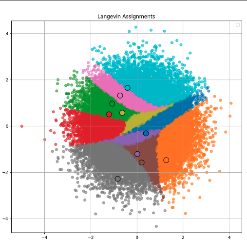
Let me illustrate it in low dimensions. Hereafter is what happens when the score is perfectly estimated: the data are 5 Dirac massses (the five black crosses), the video shows the trajectory of random points sampled from a Gaussian distribution. In this configuration, the score is accessible in close form, so the simulation is exact up to the time discretization of the Runge-Kutta scheme. All the points at final time are (almost) equal to one of the five initial points. I also illustrate below the estimation of the score using the entropic self-transport (see [Mordant 2024]) in the usual diffusion model. This estimation can be interpreted as a clever adaptive kernelized estimation of the score. I was not able to generate new unseen digits by using this relatively non-parametric estimation of the score. On the left, the generated digits, on the right, the closest (in an $L^2$ sense) digit in the database.
 |
 |
 |
 |
In the ML literature, this fact is called memorization, which is, in some sense, the opposite of generalization. On the other hand, if the estimation of the score is poor, the obtained generative model gives very unplausible images. For instance, if one uses a simple convolutional neural network to estimate the score, the resulting generative model is very poor. Therefore, one needs a sufficiently expressive class of neural networks to estimate the score, but not too expressive otherwise memorization occurs. It appears that some error (for instance early stopping of the flow) has to be made to deviate from the training samples. The backbone of the first diffusion models was a UNet with a bottleneck of attention, probably capturing correlations at different scales. More expressive models can be used such as transformers to produce good results.
My understanding, after the breakthrough paper [Song et al. 2021], was that the architecture biases were key to the success of the method.
More generally, I am still surprised by how efficient these architectures are able to capture the space of natural images and this is not explained by the mathematical theory behind diffusion models, which in my opinion, facilitate the learning of the manifold (very unsmooth though) of natural images when using neural networks. These models were and still are a very hot topic in artificial intelligence and I am sure that this community has reached a better understanding (than my own opinion which I do not share here) of what makes it work.
Diffusion models opened the door to other formulations such as flow matching. In my opinion, these developments often benefit from the optimization advantage in comparison with GANs, but their efficacy still rely on the same generalization capacity (by using adequate network architectures) mentioned above, which is not explained by the mathematical formulation at its core.
Extensions: Flow matching [Lipman et al. 2023] but other teams introduced it at the same time).
There are many ways to transport from a Gaussian distribution to an empirical distribution, such as semi-discrete optimal transport. Optimal transport selects one coupling (i.e. a probability on the product space $\mathbb R^d \times \mathbb R^d$ with the first and second marginals equal to the given distributions) among all the possible couplings between two given distributions. However, one of the key insights from optimal transport consists of intepreting a coupling as a transport! Let me explain, suppose that we are given two Dirac distributions $\delta_y$ and $\delta_z$. Any continuous path $x(t)$ starting at $y$ and ending at $z$ gives a possible “horizontal” interpolation between these two Dirac masses, which is in sharp contrast with the “vertical” interpolation $(1 - t) \delta_y+ t \delta_z$. Now, more generally, a stochastic process gives a probability on the path space $C([0,1],\mathbb R^d)$. A coupling plan does not give directly such a probability on the path space. There is an infinite number of solutions. To specify one, it is sufficient to choose an interpolation between points: this interpolation can be deterministic, choosing for instance geodesic (straight lines) interpolations or probabilistic such as a Brownian bridge, thus giving rise to Schrödinger bridges.
What is the recipe to devise a generative model using such interpolations?
Diffusion models estimate the score, that is the vector field driving the evolution of the probability measure associated with $X(t)$ the corresponding process on the path space. The corresponding PDE is a continuity equation $$ \partial_t \rho + \operatorname{div}(\rho v_t) = 0.$$ The last question is how to estimate $v_t$? Let us answer this question in the case of a probability measure supported by absolutely continuous curves, i.e. curves $\omega(t)$ that satisfy $\omega(t) - \omega(s) = \int_s^t \dot \omega(u) du$. Now, the vector field can be expressed as $v_t(x) = \mathbb E[\dot{\omega} | \omega(t) = x]$. Recall that the continuity equation is recovered by integrating against a test function: $$ \frac{d}{dt} \int_{\mathbb R^d} f(x)d\rho_t(x) = \mathbb E[\langle \nabla f(\omega(t)),\dot \omega(t)\rangle ] = \int_{\mathbb R^d} \langle \nabla f(x),\mathbb E[\dot{\omega} | \omega(t) = x]\rangle d\rho_t(x).$$
The consequence of this formula is that the estimation of the vector field $v_t$ can be performed using a Monte-Carlo method and an $L^2$ loss function in a class of adequate neural networks (similarly to equation (1))!
In comparison with diffusion models, there are at least two important differences:
- Only need to work on the finite time interval $[0,1]$.
- Any coupling plan and (deterministic) lifting on the (absolutely continuous) path space can be used.
Although I only treated the case of deterministic interpolation on the path space. The case of more general diffusion can be treated in the same way, such as the case of a Schrödinger bridge.
Although these new formulations help extending the capabilities of the generative models, they do not explain why it really works… These generalizations also rely on the idea of breaking the learning problem in small timesteps, which seems to make it easier. However, the generalization capacity of the model seems to be much more related to the expressivity bias of the architecture.
Note: This post offers an overview of the state of the field as it was a few years ago. While significant progress has been made recently, I believe my rough understanding from that time may still be useful to some of my colleagues—for example, to avoid getting lost in cutting-edge discussions on diffusion models and their technical intricacies.
Acknowledgements: I thank Eddie Aamari, Théo Lacombe and Gabriel Peyré for improving the post. I also thank Théo for sharing the video above and the picture of Langevin cells.
References.
[Sohl-Dickstein et al. 2015] Jascha Sohl-Dickstein, Eric A. Weiss, Niru Maheswaranathan, and Surya Ganguli, Deep Unsupervised Learning using Nonequilibrium Thermodynamics (International Conference on Machine Learning, 2015).
[Song and Ermon 2020] Yang Song and Stefano Ermon, Generative Modeling by Estimating Gradients of the Data Distribution (Advances in Neural Information Processing Systems, 2020).
[Song et al. 2021] Yang Song, Jascha Sohl-Dickstein, Diederik P. Kingma, Abhishek Kumar, Stefano Ermon, and Ben Poole, Score-Based Generative Modeling through Stochastic Differential Equations (International Conference on Learning Representations, 2021).
[Mordant 2024] Gilles Mordant, The entropic optimal (self-)transport problem: Limit distributions for decreasing regularization with application to score function estimation, 2024.
[Lipman et al. 2023] Yaron Lipman and Ricky T. Q. Chen and Heli Ben-Hamu and Maximilian Nickel and Matt Le, Flow Matching for Generative Modeling, 2023.